Hi-C is a sequencing-based method for profiling the genome-wide chromatin contacts. It has been widely used in studying various biological questions such as gene regulation, chromatin structures, genome assembly, etc. The Hi-C experiments involves a series of biochemistical reactions that may introduce noises to the output. Subsequent data analysis such as read mapping also give rise to noises that affect the interpretation of the final output: a contact matrix, where each element in the matrix denotes the contact strength between any two regions of genome. Therefore, a critical step in Hi-C data analysis is to remove such noises, a step also called Hi-C data normalization.
Early days of normalization methods for Hi-C data focused on explicit factors that cause noises. Factors like cutting enzyme sites, genome mappability, GC contents make the sequencing reads unevnely distributed across the genome, thus introduce biases when calculating pairwise contacts. In light of these ideas, Imakaev et al and others propose a method cappable of handling all sources of noises “implicitly” [1]. The idea behind is actually very simple: because Hi-C is an unbiased experiments in theory, the visibility across all genomic regions should be equal. Another assumption is that all biases of a Hi-C experiments are one-dimensional and factorizable. Based on these assumption, a natural solution is to factorize the raw contact matrix into a multiplication of two 1D biases and a normalized matrix whose rows and columns summed up to a same value.
The method proposed by Imakaev is also known as matrix balancing in matrix theory. Matrix balancing is an old mathematical question dated back to one century ago. Many matrix balancing methods have been developed including vanilla coverage (VC), Sinkhorn & Knopp (SK), and Knight & Ruiz methods (KR). VC is done by dividing each element of the matrix by its row sum and column sum to remove different sequencing coverage of each loci. VC can be considered as a single iteration of the SK method. In SK, the VC process is repeatly performed until all the rows and cols sum to the same value. S&K proves that this process will converge. Imakaev et al uses the standard SK method.
Rao et al reviewed all matrix balancing method ands introduced the KR method to Hi-C data [2]. Based on the original paper by K&R, KR method is several magnitute faster than SP, which makes it suitable for balancing high-resolution matrices. In practise, ICE impelementation of SP is also very fast even at 10kb resolution. In my experience, the speed difference between ICE and KR is neglectable. However, KR has a drawback that the KR process may not converge when the matrix is too sparse (as pointed out by Rao et al. 2014). This happened a couple of times in my research when I used juicertools to generate KR normalized matrix on a low sequencing dataset and got an empty matrix.
The algorithms for matrix balancing is actually not difficult, at least not as the mathematical theories behind it. So, how do we calculate a balanced matrix for a Hi-C contact matrix? Below I implemented VC and SP method in a short python class. This implementation is fast for small matrices.
1class HiCNorm(object):
2 def __init__(self, matrix):
3 self.bias = None
4 self.matrix = matrix
5 self.norm_matrix = None
6 self._bias_var = None
7
8 def iterative_correction(self, max_iter=50):
9 mat = np.array(self.matrix, dtype=float) ## use float to avoid int overflow
10 # remove low count rows for normalization
11 row_sum = np.sum(mat, axis=1)
12 low_count = np.quantile(row_sum, 0.15) # 0.15 gives best correlation between KR/SP/VC
13 mask_row = row_sum < low_count
14 mat[mask_row, :] = 0
15 mat[:, mask_row] = 0
16
17 self.bias = np.ones(mat.shape[0])
18 self._bias_var = []
19 x, y = np.nonzero(mat)
20 mat_sum = np.sum(mat) # force the sum of matrix to stay the same, otherwise ICE may not converge as fast
21
22 for i in range(max_iter):
23 bias = np.sum(mat, axis=1)
24 bias_mean = np.mean(bias[bias > 0])
25 bias_var = np.var(bias[bias > 0])
26 self._bias_var.append(bias_var)
27 bias = bias / bias_mean
28 bias[bias == 0] = 1
29
30 mat[x, y] = mat[x, y] / (bias[x]*bias[y])
31 new_sum = np.sum(mat)
32 mat = mat * (mat_sum / new_sum)
33
34 # update total bias
35 self.bias = self.bias * bias * np.sqrt(new_sum / mat_sum)
36
37 self.norm_matrix = np.array(self.matrix, dtype=float)
38 self.norm_matrix[x, y] = self.norm_matrix[x, y] / (self.bias[x] * self.bias[y])
39
40 def vanilla_coverage(self):
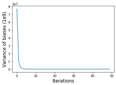
41 self.iterative_correction(max_iter=1)The idea behind above algorithm is that we start by setting the biases to the sums of each row of the matrix, and dividing each matrix element by its row- and column-wise biases. The two steps are repeated until convergence criteria are met. We can use the variance of the biases (self.bias) to monitor the convergence of the balancing process (Figure shown below).
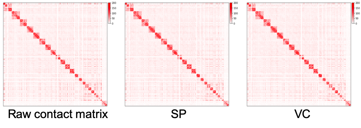
The raw contact matrix, matrices normalized by SP method and VC method are plotted as heatmaps as below. We can see that regions away from diagonal in the normalized matrices are cleaner than the raw matrix, but we can barely see the difference between SP and VC method. In practice, we pre-filter rows with very small values before normalization. The above script filters out rows whose sums fall below the 15 quantile of all row sums by setting elements of these rows to be zero.
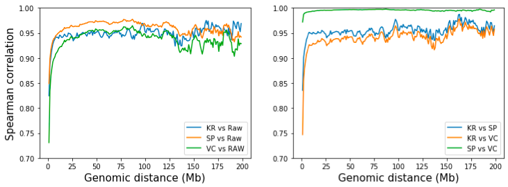
However, we can quantify the difference of SP and VC normalized methods by examining the correlation of contacts separated by the same distances. To do this, we extract and calculate the correlation of the d-th diagonal of the two matrices, where d is the distance (at bins) of two genomic regions. From the figure below, while all three methods resemble raw matrix at long distance (>10 Mb), SP is slightly more similar to raw matrix. Pairwise comparison of three methods shows that SP and VC are highly similar given that they’re only differed by number of iterations. KR resembles SP more than VC, but the difference is neglectable. [Note: KR matrix is obtained from the .hic file with straw API].
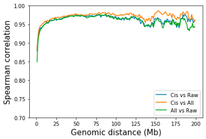
In practise, HiC normalization is done by intra-chromosome only, inter-chromosome only, or both. For intra-chromosome only, KR or ICE was done on each chromosome separately. For inter-chromosome only, the genome-wide matrix is obtained and from which the intra-chr contacts are removed. When inter-chromosome interactions are included, normalization at high resolution requires a large amount of memory. So the normalizatioln is often done on the genome-wide matrix at 25kb or 50kb resolution, as in Rao et al. A natural question is whether removing inter-chromosome contacts would have an impact on the normalization of intra-chromosome contacts? To answer this question, I performed SP normalization on All contacts vs only on intra-chromosome contacts. Again, the difference between normalized by all contacts and by only intra-chromosome contacts are really small. Juicertools and Cooler both use all contacts for normalization by default.
Conclusion
So which normalization method should I use for my data? The answer might be that it really doesn’t matter. As shown by Rao et al and our analysis, there are high correlations observed between VC, ICE(SP), KR and a couple of other matrix balancing method. Rao et al further point out that the loop calls are not affected by different normalization method in their study. They even show that loops were nearly the same when peaks were called on raw data, which makes me question whether we need matrix normalization or not. Although Rao and others did mention that VC tends to over-correct the contact map and proposed VCSQ to supplement VC, I have not seen anyone show clear evidences that KR/ICE are superior to VC/VCSQ. The pros and cons for each method are summarized as below:
| Method | Pros | Cons |
|---|---|---|
| VC/VCSQ | faster? | over-correction |
| ICE (SP) | stable? | slower? |
| KR | fastest? esp. for high-res maps | unstable for low-res maps |
In conclusion, I would still recommend normalization as part of the best pratise. Choosing KR or ICE is largely depending on the pipeline you use(Juicertools or Cooler), but if you have a relatively low sequencing depth, I would recommend ICE as it guarantees convergence.
Code availability
All codes used for this post can be found: https://github.com/dearxxj/genomics_tools/blob/master/HiC_Normalization/HiC-normalization.ipynb
Reference:
[1]. Imakaev et al. Iterative correction of hi-c data reveals hallmarks of chromosome organization. Nature Method. 2012.
[2]. Rao et al. A 3D Map of the Human Genome at Kilobase Resolution Reveals Principles of Chromatin Looping. Cell. 2014.